Executive Summary

Table of Contents

Introduction

EROI and Emergy

Tables of EROI

The Effect of Diminishing EROI on Total Energy Budget and GDP

The Effect of Political Economy on Total Energy Budget and EROI

The Relation of Energy to Money

Introduction

The material in this essay consists principally of material from the appropriate sections of the rest of the paper.

EROI and Emergy

We shall refer to the figure below in the discussion of the emergy balance.

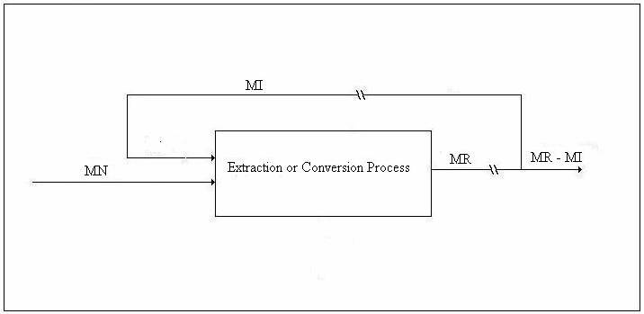
Figure 4.  Drawing for Emergy Balance

Let MN be the emergy of the work supplied by Nature, MR the emergy of the immediate energy product, and MI the emergy of the energy investment stream.  Let λ_N be the transformity of the energy supplied by Nature and λ_R the transformity of the immediate energy product (as opposed to MR – MI, the emergy delivered to the economy).  The transformity, λ_i, is the number of kWhrs of single-phase, 60 Hz, 110-volt AC electricity one can obtain from 1 kWhr of energy source i by an efficient process.  Thus, 1.0 kWhrs of single-phase, 60 Hz, 110-volt AC electricity is my (arbitrary, but well-defined) choice for the unit of emergy and λ_i is an electricity-based transformity.  Then,

where  EN is the availability provided by Nature, normally free of charge; ER is the availability of the energy returned; and EI is the availability of the energy invested.  Availability or available energy is internal energy plus pressure times volume minus the temperature of the environment times the entropy.  EROI, the ratio of (available) energy returned to (available) energy invested, is denoted β, and μ is the available energy from Nature per unit of available energy returned.  The emergy balance leads quickly to the fundamental relation between these quantities:

This relation can be used to find any one of the four variables λ_N, λ_R, μ, or β in terms of the other three.  The special cases of extraction and conversion are considered in “Balance Equations for Energy Extraction and Conversion”.

Tables of EROI

On Sheet 4 of both spreadsheets five different EROIs for each political economy and for two levels of conservation are tabulated below and to the right of DN68:

The five types of EROI are as follows:

1.      EROI^o.  The energy invested (EI) is the direct energy overhead of the energy sector.

2.      EROI¹.  EI¹ includes, in addition to the direct energy overhead, the indirect energy costs associated with the energy overhead of the manufacturing and transportation portions of the overhead of the energy sector but not the overhead due to commerce.

3.      EROI².  EI² includes, in addition, the overhead due to the activities of commerce in connection with the sale of energy.

4.      EROI³.  EI³ includes, in addition, the consumption of energy associated with that portion of the salaries paid to the energy sector in excess of what they would have been if no one earned more than the workers do.  This is thought to account for over-consumption associated with profit taking in connection with the sale of energy.

5.      EROI⁴.  EI⁴ includes, in addition, the consumption of energy by the workers in the energy sector and the pro-rata shares of the energy expenses of the workers and managers in other sectors insofar as they support the energy sector.

The four political economies are as follows:

1.         The Base Case (BC) is a steady-state idealization of an American-style market economy.

2.         The No-Managers Case (NM) is a steady-state idealization of an American-style market economy with managers, presumably chosen by the workers from among themselves, who get paid the same as workers, which reduces energy consumption.  The expression No-Managers, then, is not particularly well-chosen.  I suppose this is an idealization of market communism.

3.         The No-Commerce Case (NC) is a planned economy that has a negligible energy  overhead but that has a commissar class which enjoys the same privileges as managers do in a market economy.  Perhaps it is an idealized Soviet economy.

4.         The No-Commerce-No-Managers Case (NCNM) has a give-away economy with no energy overhead and with the same income for everyone whether they work or not.  It is most like the natural economy advocated in On the Preservation of Species, “Energy in a Natural Economy”, “On the Conservation-within-Capitalism Scenario”, and “The Demise of Business as Usual” all of which are hyperlinked to http://www.dematerialism.net/.

The two levels of conservation are as follows with the second level split:

1.         Conservation Level 1 is no conservation at all or rather only such conservation measures as have been implemented in the US American economy at the present time.

2.         Conservation Level 2 is any conservation factor, ψ, less than 1.0 in the linear relations that adjust the levels of consumption of the four commodities between their values in the Base Case, which represents the US economy at the present time, and a fraction φ_i of the present value where φ_A = 0.2, φ_R = 0.3, φ_M = 0.1, and φ_T = 0.1; and that adjusts the energy overhead for each of the four sectors C, A, M, and, T between their values for the Base Case and a fraction ξ_i of the present value where ξ_C = 0.5, ξ_A = 0.1, ξ_M = 0.5, ξ_T = 0.1.

2a.       With an EROI^o = 21 for a fossil-fuel economy, the conservation factor ψ is reduced until the energy budget in the Base Case has been reduced to Pimentel’s value for Maximum Renewables. 

2b.       With an EROI^o = 3 for a renewable-energy economy, the conservation factor has been reduced until the energy budget for the No-Commerce-No-Managers (NCNM) Case corresponding to the Natural Economy has been reduced to Maximum Renewables.

The final EROI calculations are done on Sheet 4 in the block spanned by DN48 and DR66.  The principal computations are in Columns GM through IV, the end of the spreadsheet.

The Effect of Diminishing EROI on Total Energy Budget and GDP

Chart 2 illustrates the effect of reducing the EROI due to substituting a less efficient technology for the technology that preceded it chronologically.  One sees the total energy budget, E, approaching infinity as EROI diminishes toward 1.0.  In this paper, I have defined Energy Returned to be the total energy extracted or produced.  This is the sum of the energy delivered and the energy invested.  An alternative definition counts only the energy delivered.  This has the advantage that it is easily computed in practice.  For example, if a Concentrated Solar Power (CSP) installation is rated at 500 MW with an operating factor of 0.3 and a plant life of 30 years, ER = 500 MW · 0.000001 TW/MW · 0.3 · 30 years = 0.012 terawatt-years = 39 billion kilowatt-hours.  If the alternative definition is used, each of the EROIs is reduced by exactly 1.0 and the total energy budget approaches infinity as EROI-1 approaches zero.  This result is illustrated graphically in Chart 2 on each of the two spreadsheets http://www.dematerialism.net/Mark-II-Economy.xls and http://www.dematerialism.net/Mark-II-Economy-CSP.xls.  Chart 2, above, is an older version of the chart that no longer corresponds to either of the spreadsheets but illustrates the effects qualitatively and is nicer looking than the current versions.

The Effect of Political Economy on Total Energy Budget and EROI

In this copy of Chart 1 from Mark-II-Economy-CSP.xls, one sees that E_BC > E_NM > E_NC > E_NCNM. 

 

This illustrates the reductions in energy consumption that can be expected with the specified changes in political economy; but, a little more is needed to justify this essay by making the case for political change sufficiently compelling.

The savings indicated for a move from the Base Case (BC), which is an ideal steady-state, market economy, to the No-Managers Case (NM), which is an ideal sort of market communism, will exceed the savings from BC to any realistic actual implementation of a steady-state market economy by definition.  The same is true for moves from NM to the No-Commerce Case (NC) and from NC to the No-Commerce-No-Managers Case (NCNM).  Let us characterize the worst-case scenario for each case with an asterisk and the best-case idealization with an unembellished symbol since the cases in the model are the best-case idealizations.  Thus, E_BC* > E_BC, E_NM* > E_NM, E_NC* > E_NC, and E_NCNM* > E_NCNM or, more likely, E_NCNM* = E_NCNM.  But, the energy costs of commerce are “the elephant in the living room” as discussed and computed in “Energy in a Natural Economy”; therefore, E_NM > E_NC*.  Moreover, an idea that is central to Dematerialism is the following:  If the core aspects of two economic systems are the same, the system that does not tolerate the profit motive will be much more efficient than the system in which inequality of income and wealth is permitted.  Therefore, if we forego the possibility of validating Dematerialism with this result, as that would lead to circular reasoning, we may assume that E_BC > E_NM* and E_NC > E_NCNM*.  So, for identical standards of living,

E_BC* > E_BC > E_NM* > E_NM > E_NC* > E_NC > E_NCNM* > E_NCNM .                          Principal Relation

Practically, the entire book On the Preservation of Species is devoted to reasons why dispensing with the profit motive will have felicitous effects.  The Principal Relation is the most important result of this paper.  It compels one to consider political change in the wake of Peak Oil.  However, further testimony is provided by Experiment 4 on Sheet 4 below and to the right of DN94:

 

 

In Experiment 4,  with the conservation factor ψ = 0.545142, the total energy budget for the capitalist economy as represented by the Base Case is just equal to Pimentel's figure for Maximum Renewables whereas the Natural Economy as represented by the No-Commerce-No-Managers Case has an energy budget of 38.884% of that modest figure, an energy budget that could be met by local private efforts.   With the switch to renewables reducing the basic EROI to 3.0, the Natural economy is at Maximum Renewables with ψ = 0.635064; but, the capitalist economy is still consuming 220.62% of Maximum Renewables.  This example was taken from the constant-sector-population spreadsheet.

Finally, it is important to notice in Chart 1 that EROI improves with energy savings; therefore, a primary energy technology that fails in a capitalist economy because of too low an EROI may succeed in a Natural Economy.

The Relation of Energy to Money

For an entire economy, for a median transaction within that economy, or for a transaction of such great scope that such concentrations within particular energy consuming sectors as may exist in one phase or another of the transaction tend to get smoothed out, the energy consumed is approximately equal to the dollar amount of the total cost of the transaction times the Total National Energy Budget (E) over Gross Domestic Product (GDP) ratio (E/GDP) that is tabulated in the DOE database for every country and for every year – within limits. The purchase and operation of a custom-built nuclear power plant is just such a transaction of extremely broad scope to which this type of analysis might apply.

Exercise 1a in http://www.dematerialism.net/Mark-II-Money.html validates the idea of getting a good approximation to the energy invested from the total cash invested from the inception of the project until the last vestiges have been cleaned up after the life cycle of the installation has come to a close.  We show that, if an investment is distributed among the commodities in the same proportion as consumer spending is distributed, the increase in the Total Energy Budget, ΔE, will be precisely the increase in the GDP resulting from the investment times (E/GDP)_o.  The reader should understand that the fraction of the investment that is made in commodity i is m_i, which is equal to the cash spent by consumers on commodity i divided by the total cash spent by consumers.  Also, very good agreement was found in Experiment 1b for a distribution over the RUs, MUs, and TUs (but not AUs) in the proportion that they are distributed over the economy at large; and, in Experiment 1c, order of magnitude agreement was found for a distribution over just manufacturing and transportation.

One often sees a figure for the money to be invested and almost never a figure for the energy to be invested.  Hopefully, that will change due to our efforts and the efforts of many others.

Thomas L. Wayburn

Houston, Texas

October 17, 2006